The “Climate Crisis”, or “Climate Emergency”, or climate “Existential Threat” is an international political construct based on the projections of an ensemble of numerous, unverified climate models run with ranges of input factors, since the actual values of these input factors are unknown. The perception of crisis is a creature of political science, not hard science.
The principal factor on which the concern is focused is a reported increase in global average temperature of 1°C over the 120 year period since 1900 and the potential global adverse impacts of another 0.5-1.0°C increase beyond current levels over some undefined future period.
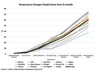
Very little effort has been put forth by the consensed climate science community to provide perspective regarding the current and projected future temperature increases. However, Dr. Richard Lindzen recently made a presentation on “The Imaginary Climate Crisis” in which he included the following graph focused on placing the purported temperature change in perspective. The graph shows the magnitude of regular, shorter term temperature changes in fourteen cities in the contiguous United States. Analysis of the same temperature changes in other cities globally would produce differing numbers but display the same general patterns.
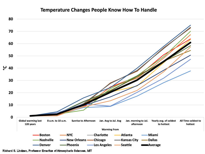
The first segment on the horizontal axis shows the global average temperature anomaly over the period 1900-2020 as approximately 1°C.
The second segment on the horizontal axis shows the individual city and average temperature change which commonly occurs in these cities over the two-hour period from 8 am to 10 am on any given day, which ranges from approximately 1-5°C, or up to 5 times the global average temperature increase over the past 120 years of concern to global politicians.
The third segment on the horizontal axis shows the typical “sunrise to afternoon” temperature change in these cities on any given day, which ranges from approximately 7-17°C, or 7-17 times the global average temperature increase over the past 120 years.
The fourth segment on the horizontal axis shows the typical difference between the January average temperature and the July average temperature in each of the cities, which ranges from approximately 9-28°C, or 9-28 times the global average temperature increase of concern to climate alarmist politicians.
The fifth segment on the horizontal axis shows the typical temperature difference between a January morning and a July afternoon in each city, which ranges from approximately 18-40°C over the six month period, or 18-40 times the temperature increase of concern to climate alarmist politicians.
The sixth segment on the horizontal axis shows the typical temperature difference between the yearly average hottest and coldest temperature in each of the cities, which ranges from approximately 30-60°C over the average year, or 30-60 times the temperature increase of concern.
The seventh segment on the horizontal axis shows the temperature difference between the warmest and the coldest temperatures ever recorded for each of the cities, which ranges from approximately 38-75°C, or 38-75 times the maximum temperature difference of record.
Clearly, the reported global annual average temperature increase typically attributed to increased atmospheric CO2 concentrations pales in comparison to typical hourly, daily and seasonal temperature changes and to the record temperature difference for each city. Also, since approximately 60% of the reported global annual average near-surface temperature increase is an increase in the nightly low temperature while only approximately 40% is an increase in the daily high temperature, it seems unlikely that people would be unable to handle the future temperature increases of concern to climate alarmists.


 The Right Insight is looking for writers who are qualified in our content areas. Learn More...